CWT in PCSEL

3D-CWT: the repository

3D-CWT is our open-source Python implementation of three-dimensional coupled-wave theory for square-lattice photonic-crystal surface-emitting lasers (PCSELs). The current release is 1.3.1. Starting from a layer stack and a photonic-crystal unit cell, the optical solver calculates the vertical guided mode, the four-wave coupling matrix, and the modes of a finite cavity using NumPy and SciPy.

The calculation follows this sequence:

Layer stack and hole geometry → averaged vertical waveguide → Fourier coefficients and outgoing Green functions → four-wave coupling matrix → finite-cavity eigenmodes.

This post explains that sequence, beginning with 2D CWT and then introducing the vertical structure and surface radiation in 3D CWT. The final section presents results from the 1.3 series. The released optical solver covers lossless-material, scalar TE calculations on a square lattice; carrier transport and above-threshold laser dynamics are outside its scope.

The earlier version of this post is retained as a historical note. The equations below use the conventions of the current implementation.

Introduction to coupled-wave theory

A PCSEL combines in-plane distributed feedback with out-of-plane diffraction. Near the second-order Bragg condition of a square lattice, four counterpropagating guided waves dominate the resonant field. Their interference determines the band-edge modes, while scattering into the normal direction provides surface emission.

Resolving every unit cell of a large-area cavity with FDTD or FEM can be expensive. CWT separates the fast lattice-scale oscillation from the slowly varying cavity envelope. The unit-cell and vertical calculations determine a small coupling matrix; the finite-device calculation then solves for four envelopes across the aperture.

Sakai, Miyai, and Noda developed a square-lattice TE coupled-wave model in 2006.^[1] Liang and co-workers subsequently incorporated the vertical waveguide and radiation into a 3D formulation.^[2] Liang’s doctoral thesis gives the detailed derivation and finite-cavity examples used here.^[3] Later work by Inoue and co-workers further organized Hermitian and non-Hermitian couplings for large-area PCSEL design.^[4]

Bloch’s theorem and conventions

For an in-plane periodic dielectric, a Bloch field is a plane wave multiplied by a lattice-periodic function. With time dependence $\exp(+\mathrm{i}\omega t)$, write

$$\mathbf E(\boldsymbol\rho,z) =\mathrm{e}^{-\mathrm{i}\mathbf k_\parallel\cdot\boldsymbol\rho} \mathbf u_{\mathbf k_\parallel}(\boldsymbol\rho,z), \qquad \boldsymbol\rho=(x,y).$$

For a square lattice of period $a$, the reciprocal vectors are

$$\mathbf G_{m,n}=\beta_0(m,n),\qquad \beta_0=\frac{2\pi}{a}.$$

The relative permittivity has the expansion

$$\epsilon(\boldsymbol\rho,z) =\bar\epsilon(z)+\sum_{(m,n)\ne(0,0)} \xi_{m,n}(z)\mathrm{e}^{-\mathrm{i}\mathbf G_{m,n}\cdot\boldsymbol\rho},$$

$$\xi_{m,n}(z)=\frac{1}{a^2}\int_{\mathrm{cell}} \epsilon(\boldsymbol\rho,z) \mathrm{e}^{+\mathrm{i}\mathbf G_{m,n}\cdot\boldsymbol\rho}\,\mathrm{d}^2\rho, \qquad (m,n)\ne(0,0).$$

Here $\bar\epsilon$ is the cell-averaged relative permittivity. The sum includes orders such as $(1,0)$ and $(0,1)$; only the pair $(0,0)$ is excluded. For real materials, $\xi_{-m,-n}=\xi_{m,n}^*$. Hole shape, filling fraction, and position enter through these coefficients.

At the folded $\Gamma$ point, the four basic harmonics are

$$\mathcal B=\{(1,0),(-1,0),(0,1),(0,-1)\}.$$

All four have in-plane wavenumber magnitude $\beta_0$. The $(0,0)$ harmonic describes normal radiation, and orders with $m^2+n^2>1$ are the auxiliary harmonics.

Coupled-wave theory

2D CWT

The in-plane wave equation

First consider a dielectric structure invariant along $z$. For TE polarization, the electric field lies in the $x$–$y$ plane and the magnetic field has a scalar component $H_z$. In a nonmagnetic medium,

$$\frac{\partial}{\partial x} \left(\frac{1}{\epsilon}\frac{\partial H_z}{\partial x}\right) +\frac{\partial}{\partial y} \left(\frac{1}{\epsilon}\frac{\partial H_z}{\partial y}\right) +k_0^2H_z=0,\qquad k_0=\frac{\omega}{c}.$$

For the periodic problem at $\Gamma$, expand

$$H_z=\sum_{\mathbf p}h_{\mathbf p} \mathrm{e}^{-\mathrm{i}\mathbf G_{\mathbf p}\cdot\boldsymbol\rho}, \qquad \frac{1}{\epsilon}=\sum_{\mathbf p}\eta_{\mathbf p} \mathrm{e}^{-\mathrm{i}\mathbf G_{\mathbf p}\cdot\boldsymbol\rho}.$$

Substitution gives the Fourier-space equations

$$\sum_{\mathbf q} (\mathbf G_{\mathbf p}\cdot\mathbf G_{\mathbf q}) \eta_{\mathbf p-\mathbf q}h_{\mathbf q} =k_0^2h_{\mathbf p}.$$

The inverse-permittivity coefficients $\eta_{\mathbf p}$ belong to this magnetic-field formulation. They should not be interchanged with the permittivity coefficients $\xi_{\mathbf p}$ used in the electric-field formulation below.

From many harmonics to four waves

Near Bragg resonance, retain the four basic harmonics explicitly:

$$\begin{aligned} H_z\simeq{}&h_{+x}\mathrm{e}^{-\mathrm{i}\beta_0x} +h_{-x}\mathrm{e}^{+\mathrm{i}\beta_0x}\\ &+h_{+y}\mathrm{e}^{-\mathrm{i}\beta_0y} +h_{-y}\mathrm{e}^{+\mathrm{i}\beta_0y} +\text{auxiliary harmonics}. \end{aligned}$$

The auxiliary harmonics mediate additional scattering paths. In the early 2D model, the four diagonal orders $(\pm1,\pm1)$ provide important indirect coupling between the $x$- and $y$-propagating basic waves. More generally, partition the Fourier system into basic and auxiliary amplitudes:

$$\begin{pmatrix} M_{BB}&M_{BH}\\ M_{HB}&M_{HH} \end{pmatrix} \begin{pmatrix}h_B\\h_H\end{pmatrix}=0.$$

Eliminating $h_H$ gives

$$\left(M_{BB}-M_{BH}M_{HH}^{-1}M_{HB}\right)h_B=0.$$

This is the central coupled-wave reduction: direct scattering and paths through eliminated harmonics both contribute to an effective four-wave problem. A slowly varying envelope approximation then retains first derivatives of the basic amplitudes and neglects their second derivatives.

The 2D model explains in-plane feedback and band splitting. Its $z$-invariant geometry has no upper or lower radiation boundary. Surface emission must be supplied by an additional model; a quantitative treatment of the layer stack requires the 3D extension.

3D CWT

1. Solve the averaged vertical waveguide

In a multilayer PCSEL, the four basic waves share a reference guided profile $\Theta_0(z)$. It satisfies

$$\frac{\mathrm{d}^2\Theta_0}{\mathrm{d}z^2} +\left[k_0^2\bar\epsilon(z)-\beta^2\right]\Theta_0=0, \qquad \int_{-\infty}^{+\infty}|\Theta_0(z)|^2\,\mathrm{d}z=1.$$

The normalization includes the evanescent tails in both claddings. For a specified period, our examples determine the reference frequency by solving

$$\beta_{\mathrm{fundamental}}(k_0)=\beta_0=\frac{2\pi}{a}.$$

Define the electric-field envelope vector in the fixed order

$$\mathbf V=(R_x,S_x,R_y,S_y)^{\mathsf T}.$$

Its basic-wave contribution is

$$\begin{aligned} E_y^{(B)}&=\Theta_0(z) \left[R_x(x,y)\mathrm{e}^{-\mathrm{i}\beta_0x} +S_x(x,y)\mathrm{e}^{+\mathrm{i}\beta_0x}\right],\\ E_x^{(B)}&=\Theta_0(z) \left[R_y(x,y)\mathrm{e}^{-\mathrm{i}\beta_0y} +S_y(x,y)\mathrm{e}^{+\mathrm{i}\beta_0y}\right]. \end{aligned}$$

Thus $R_x,S_x$ multiply $E_y$, whereas $R_y,S_y$ multiply $E_x$. These are electric-field amplitudes, with a different basis convention from the preceding $H_z$ expansion.

2. Calculate radiation and auxiliary fields

The radiation and auxiliary harmonics generally have vertical profiles different from $\Theta_0$. For each in-plane order, introduce an outgoing scalar TE Green function:

$$\left[\frac{\mathrm{d}^2}{\mathrm{d}z^2} +k_0^2\bar\epsilon(z)-|\mathbf G_{m,n}|^2\right] G_{m,n}(z,z')=-\delta(z-z').$$

It is continuous across the source and material interfaces, has a derivative jump of $-1$ at $z=z'$, and satisfies outgoing or decaying conditions in the outer halfspaces. For a homogeneous medium,

$$G_{m,n}(z,z')=-\frac{\mathrm{i}}{2k_{z,mn}} \mathrm{e}^{-\mathrm{i}k_{z,mn}|z-z'|}, \qquad k_{z,mn}^2=k_0^2\bar\epsilon-|\mathbf G_{m,n}|^2,$$

with the outgoing/decaying branch chosen for the stated time convention. The package uses the full layered kernel, including interface reflections. The homogeneous expression is useful for understanding the approximation used in the thesis comparison.

A basic wave produces a polarization source proportional to $\xi\Theta_0$. The Green function propagates that source vertically; a second Fourier coefficient scatters the induced field back into a basic wave. The resulting overlaps have the form

$$\iint \Theta_0^*(z)\,\xi_{\mathrm{out}}(z) G_{m,n}(z,z')\, \xi_{\mathrm{in}}(z')\Theta_0(z')\, \mathrm{d}z'\mathrm{d}z.$$

The receiver coefficient at $z$ and source coefficient at $z'$ remain distinct, particularly when more than one layer is patterned. For auxiliary orders, the electric-field reconstruction also contains a local longitudinal term from the divergence constraint. Both the Green-mediated and local terms enter the high-order coupling.^[3:1]

3. Assemble the coupling matrix

Projecting the electric-field equations onto $\Theta_0$ gives

$$C=C_{\mathrm{1D}}+C_{\mathrm{rad}}+C_{\mathrm{2D}}.$$

All three matrices have units of inverse length. The names describe the scattering paths:

• $C_{\mathrm{1D}}$: direct feedback between counterpropagating waves on the same axis, using Fourier orders such as $(2,0)$ and $(0,2)$.
• $C_{\mathrm{rad}}$: scattering through the normal-radiation harmonic $(0,0)$, giving both a frequency shift and radiative loss.
• $C_{\mathrm{2D}}$: coupling through the auxiliary orders $m^2+n^2>1$, including both their Green-mediated and local contributions.

For example, the direct coupling from $S_x$ to $R_x$ is

$$(C_{\mathrm{1D}})_{12} =-\frac{k_0^2}{2\beta_0} \int\xi_{2,0}(z)|\Theta_0(z)|^2\,\mathrm{d}z.$$

To display the radiation term compactly, let $\mathbf b_i$ run over $\mathcal B$ in the order of $\mathbf V$, and let $\mathbf e_i=(\hat{\mathbf y},\hat{\mathbf y},\hat{\mathbf x},\hat{\mathbf x})_i$. Then

$$\begin{aligned} (C_{\mathrm{rad}})_{ij} ={}&-\frac{k_0^4}{2\beta_0}(\mathbf e_i\cdot\mathbf e_j)\\ &\times\iint \Theta_0^*(z)\xi_{\mathbf b_i}(z) G_{0,0}(z,z')\xi_{-\mathbf b_j}(z')\Theta_0(z') \,\mathrm{d}z'\mathrm{d}z. \end{aligned}$$

Similarly, let $\mathbf E_{\mathbf h}^{(j)}(z)$ be the auxiliary field induced by a unit amplitude of basic wave $j$, within the retained-order elimination. Its contribution is

$$(C_{\mathrm{2D}})_{ij} =-\frac{k_0^2}{2\beta_0} \sum_{\mathbf h\in\mathcal H_D} \int\Theta_0^*(z)\xi_{\mathbf b_i-\mathbf h}(z) \mathbf e_i\cdot\mathbf E_{\mathbf h}^{(j)}(z)\,\mathrm{d}z,$$

$$\mathcal H_D=\{(m,n): |m|,|n|\le D,\ m^2+n^2>1\}.$$

These expressions show where the geometry, vertical confinement, and outgoing boundary conditions enter. The component formulas are given in thesis Eqs. (3.27)–(3.35); the corresponding implementation is in src/cwt3d/coupling.py.

At $\Gamma$ in an infinite periodic structure, the envelope derivatives vanish and the problem reduces to

$$C\mathbf V=\Lambda\mathbf V,\qquad \Lambda=\delta+\mathrm{i}\alpha.$$

The four eigenvectors describe the four band-edge families. Here $\delta$ is the linearized Bragg detuning, conventionally $\delta=(\beta^2-\beta_0^2)/(2\beta_0)\simeq\beta-\beta_0$, and $\alpha$ is the amplitude-loss coefficient. The corresponding power-loss coefficient is $2\alpha$. An open, radiating structure has a non-Hermitian $C$ even when its constituent materials are lossless. Under the lossless-material, evanescent-auxiliary conditions, the nonradiative contributions are Hermitian.

4. Solve the finite-cavity envelopes

For a finite square aperture, the four amplitudes vary across the device:

$$\Lambda\mathbf V=C\mathbf V+ \mathrm{i} \begin{pmatrix} \partial_xR_x\\ -\partial_xS_x\\ \partial_yR_y\\ -\partial_yS_y \end{pmatrix}.$$

On $0\le x,y\le L$, the no-incoming-wave boundaries are

$$R_x(0,y)=0,\qquad S_x(L,y)=0,\qquad R_y(x,0)=0,\qquad S_y(x,L)=0.$$

Outgoing waves remain free at the opposite edges. Setting every component to zero on every boundary would describe a different problem.

The solver places $R_x,S_x$ on the $x$ faces of envelope cells and $R_y,S_y$ on the $y$ faces. Face averages supply the cell-center fields, and face differences supply the derivatives. After eliminating the incoming boundary unknowns, the staggered discretization gives a sparse generalized eigenproblem

$$A\mathbf v=\Lambda B\mathbf v.$$

This grid resolves the cavity-scale variation, not every lattice period. A targeted shift-invert solve finds modes near a chosen complex shift; a single such search does not enumerate all competing modes.

5. Check the power balance

Define the envelope norm

$$P=\iint_{\Omega}\mathbf V^\dagger\mathbf V\,\mathrm{d}x\mathrm{d}y.$$

The outgoing edge flux is

$$\begin{aligned} P_{\mathrm{edge}}={}&\int_0^L \left[|R_x(L,y)|^2+|S_x(0,y)|^2\right]\mathrm{d}y\\ &+\int_0^L \left[|R_y(x,L)|^2+|S_y(x,0)|^2\right]\mathrm{d}x. \end{aligned}$$

Taking the imaginary part of the integrated envelope equation gives

$$2\alpha P=P_{\mathrm{edge}} +2\iint_{\Omega}\operatorname{Im} \left(\mathbf V^\dagger C\mathbf V\right)\,\mathrm{d}x\mathrm{d}y.$$

When the auxiliary orders are evanescent and the materials are lossless, the volume term is the normal-radiation contribution. This identity separates edge leakage from surface radiation and provides an independent check of the finite discretization. With an added uniform modal gain, the threshold condition in power-gain units is $\Gamma g_{\mathrm{th}}=2\alpha+\alpha_{\mathrm i}$, where $\Gamma$ is the active-region confinement factor and $\alpha_{\mathrm i}$ represents additional internal power loss.

Results from the 1.3 series

A 70 µm circular-hole cavity

The introductory example follows Table 4.1 of Liang’s thesis: a 295 nm square lattice, circular air holes with filling fraction 0.16, and a $70\times70\ \mu\mathrm m^2$ aperture. The finite layer thicknesses are 30/64/40/40/22/118/20 nm; the corresponding indices are 3.524/3.553/3.524/3.279/3.524/$n_{\mathrm{PC}}$/3.524. The PC layer uses GaAs with index 3.524 and air with index 1. Both outer claddings have index 3.307 and are continued as homogeneous halfspaces, replacing the thesis’s listed 1.5 µm cladding segments without an additional outer interface.

The averaged PC permittivity is 10.59160384. Solving the guided-mode Bragg condition gives a reference vacuum wavelength of approximately 0.990976 µm; this is a calculated reference, not a measured lasing wavelength.

Calculated 70 µm circular-hole cavity envelope and center-line profiles

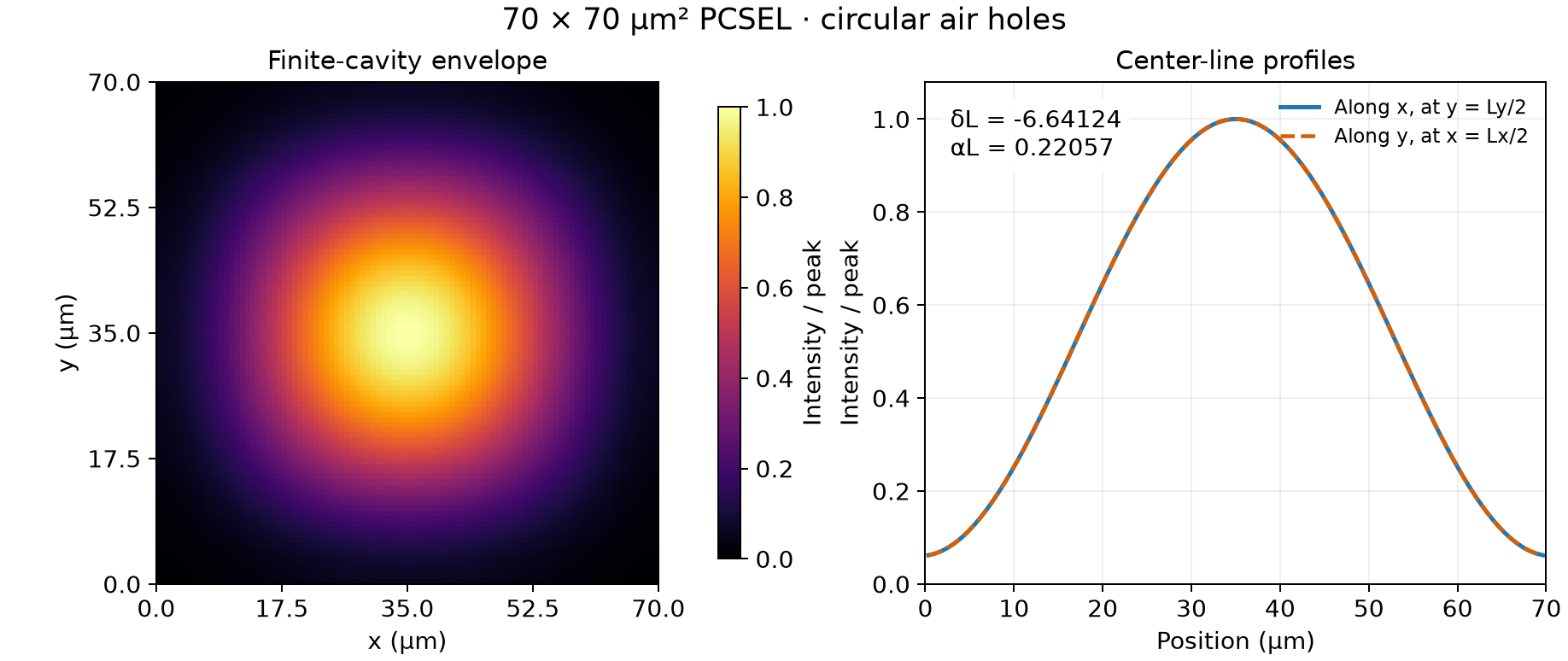
Calculated envelope intensity $I_{\mathrm{env}}=|R_x|^2+|S_x|^2+|R_y|^2+|S_y|^2$, divided by its peak, and the two center-line cuts. Controls: $N=96$, $D=32$, vertical quadrature $q=64$. The image shows the slow envelope, not unit-cell interference or optical power in watts.

For this selected mode,

Quantity	Calculated value
$\delta L$	−6.64124431
$\alpha L$	0.22057143
Total power-loss coefficient $2\alpha$	0.00630204 µm⁻¹
Edge contribution	0.00424296 µm⁻¹
Radiation contribution	0.00205908 µm⁻¹

The two loss contributions sum to $2\alpha$. This example targets one single-lobed mode near the lowest-frequency periodic band edge. The example notes and stored results provide the full structure and refinement controls.

Hole shape, filling fraction, and radiation

The Chapter 3 comparison uses a different vertical structure from the Chapter 4 finite-cavity example. It scans nine filling fractions from 0.08 to 0.24 for circular holes (CC), equilateral-triangular holes (ET), and right-isosceles-triangular holes (RIT), with $D=10$.

Three hole shapes: radiation loss and frequency versus air-hole filling fraction

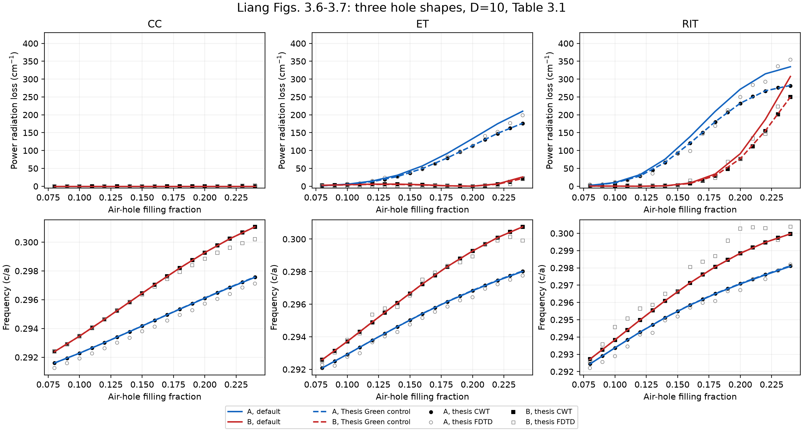
Columns: CC, ET, and RIT. Top: power radiation loss in cm⁻¹; bottom: normalized frequency $fa/c$. Solid curves are the default layered-Green calculations; dashed curves are a separate thesis-Green approximation control. Markers distinguish the thesis CWT and FDTD results, extracted from the published figures.

The circular-hole A/B modes have zero radiation loss in the infinite periodic calculation because their normal-radiation amplitudes cancel. Triangular holes alter the Fourier coefficients and the modal interference, opening radiation for these branches. The finite circular-hole cavity still radiates: spatially varying envelopes and open edges change the infinite-period cancellation condition.

The calculated frequencies closely follow the thesis CWT curves. For reference losses above 3 cm⁻¹, the default ET/RIT radiation losses have mean relative differences of approximately 14.5%/17.4% from the thesis CWT markers. The separate homogeneous-Green control moves the losses closer to those markers. This comparison isolates a modeling difference—interface reflections are retained in the default kernel—and does not establish agreement with every FDTD point.

Finite spectra and mode profiles

The next comparison returns to the Chapter 4 structure, $L=70\ \mu\mathrm m$ and filling fraction 0.16. The A–D families are identified from their fields and frequency character, rather than by selecting the four lowest-loss numerical eigenvalues.

Finite-cavity detuning-loss spectra for circular and equilateral-triangular holes

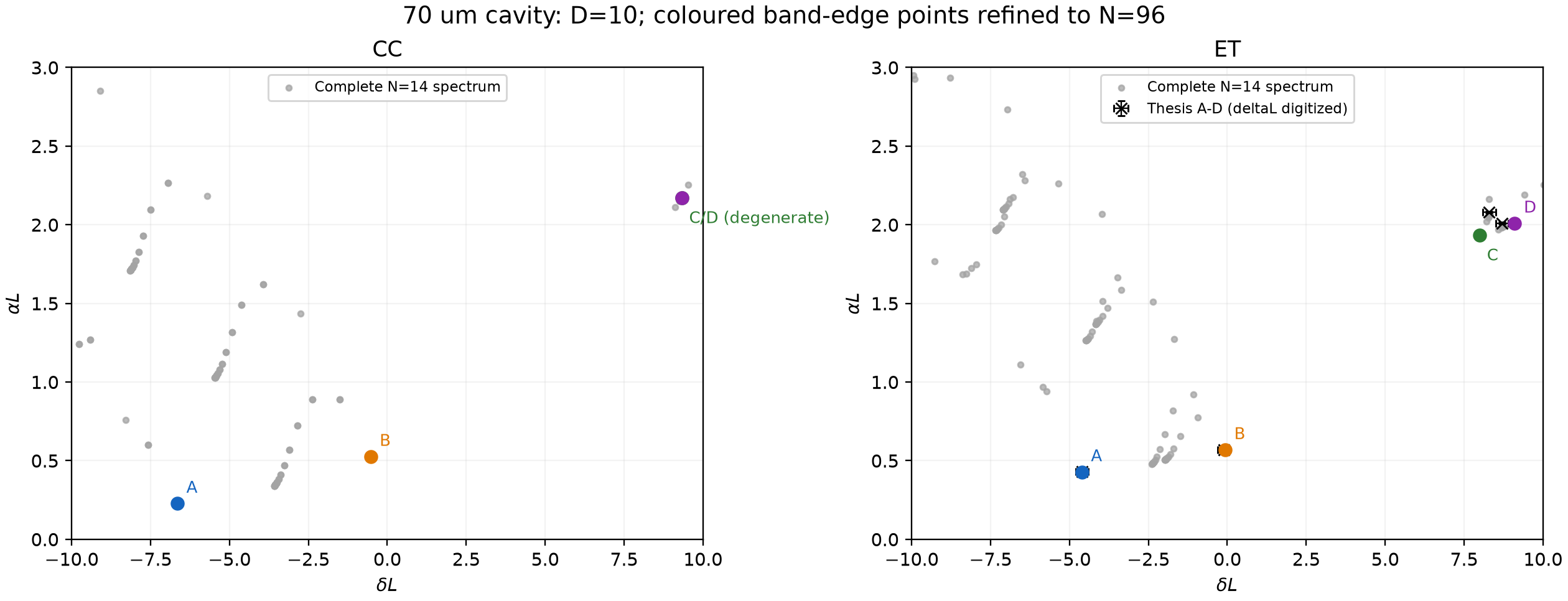
The gray cloud is the complete $N=14$ discrete spectrum. Colored A–D points are tracked to $N=96$ at fixed $D=10$. The ET panel also shows thesis reference positions; there is no corresponding thesis $\delta L$ reference in the CC panel. Axes are $\delta L$ and amplitude loss $\alpha L$.

Four finite-cavity envelope families for circular and equilateral-triangular holes

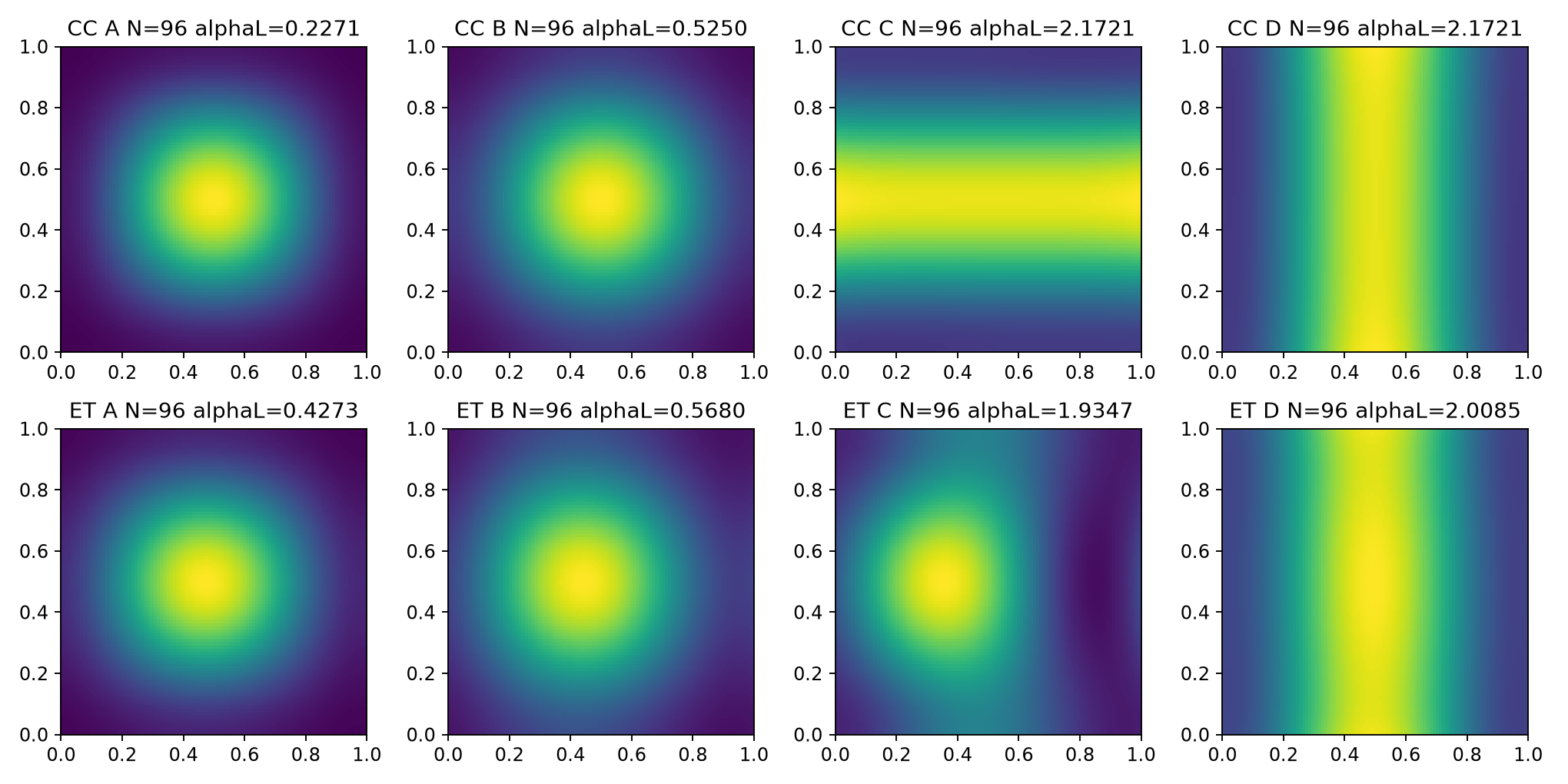
Top row: CC; bottom row: ET. Each panel shows its own peak-normalized envelope intensity on coordinates $x/L,y/L$. Controls: $D=10$, $q=32$, $N=96$. The circular-hole C/D modes form a degenerate pair; the displayed horizontal/vertical patterns are one choice of basis within that two-dimensional subspace.

The comparison with thesis Table 4.2 is:

Mode	CC: thesis $\alpha L$	CC: calculated $\alpha L$	ET: thesis $\alpha L$	ET: calculated $\alpha L$
A	0.23	0.227058	0.43	0.427323
B	0.52	0.525020	0.57	0.568033
C	2.18	2.172118	2.08	1.934732
D	2.18	2.172118	2.01	2.008507

Seven of the eight amplitude-loss thresholds differ by at most 1.3%. ET-C remains 6.98% lower than the thesis value, and the ET-C/D frequency positions also differ. Increasing the auxiliary cutoff does not remove the ET-C discrepancy. The thesis table is printed to two decimal places, so its displayed precision is separate from numerical or physical uncertainty.

The $D=10$ comparison and the introductory $D=32$ image use different cutoffs. Their CC-A values, 0.227058 and 0.22057143, correspond to those respective settings.

Cavity size and numerical refinement

Finite- and infinite-cavity A/B frequencies and losses versus cavity size

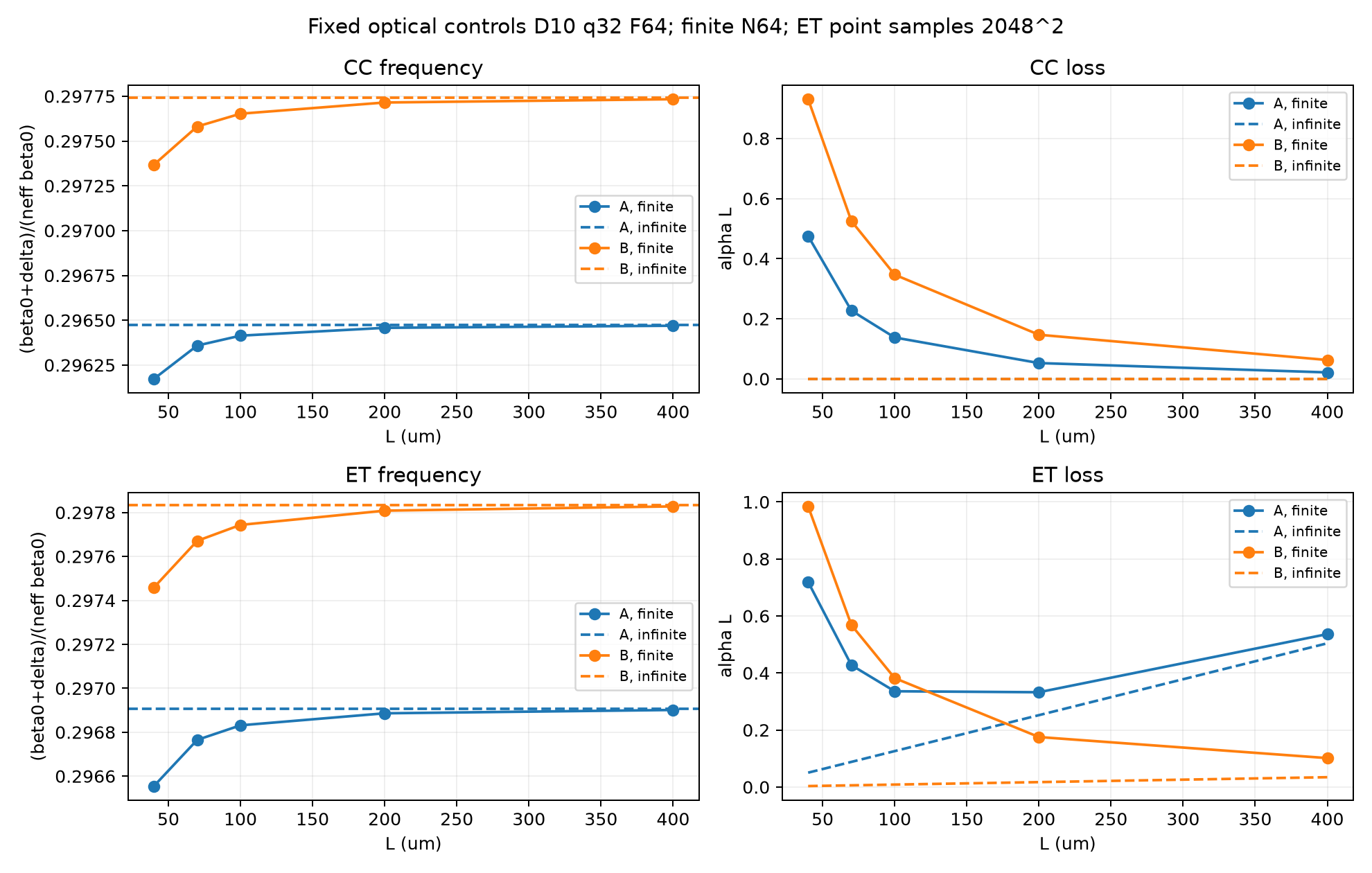
CC and ET A/B branches for sampled sizes from 40 to 400 µm. Left: normalized frequency; right: $\alpha L$. The optical controls are $D=10$, $q=32$, $F=64$, with a finite-envelope grid of $N=64$. Dashed curves show the infinite-period comparison. A separate $N=96$ calculation checks the 400 µm endpoint.

The finite-mode frequencies approach their periodic band edges as the cavity grows. For ET, A has the lower threshold at 70 µm, while B has the lower threshold at 400 µm; the ordering exchanges between the sampled 100 and 200 µm points. The size-dependent balance of edge leakage and surface radiation therefore changes which band-edge family is favored. Here the plotted loss is $\alpha L$, so its size dependence includes the normalization by $L$.

Envelope-grid refinement at fixed Fourier cutoff

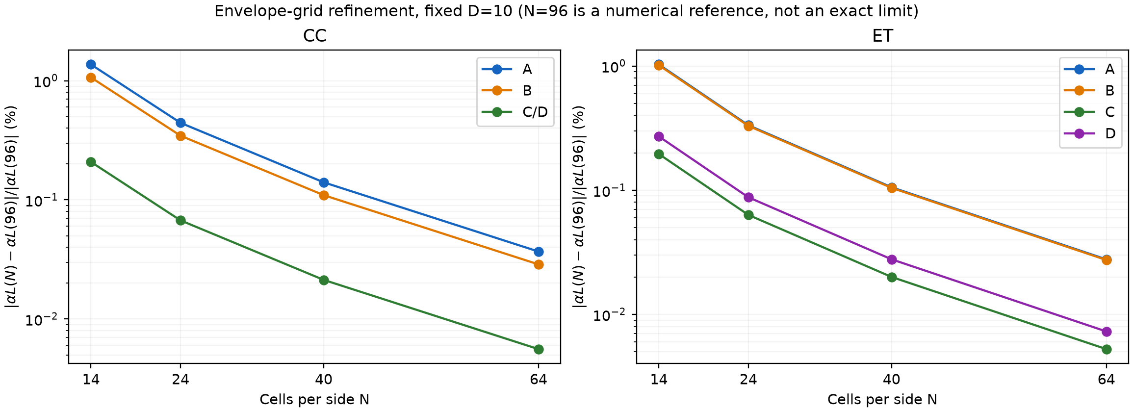
Relative changes are plotted against the $N=96$ numerical reference at fixed $D=10$. That reference is not an exact continuum solution.

The maximum $N=64\to96$ change in $\alpha L$ is 0.0368% for the eight tracked modes. Auxiliary-harmonic refinement is slower: in the Chapter 3 RIT case, B-mode radiation loss still changes by 2.93% at $D=24\to32$. For the introductory CC example, the selected mode’s $\alpha L$ changes by 0.456% over that cutoff step. Envelope-grid refinement, vertical quadrature, and Fourier truncation control different errors and must be checked separately.

The full reproduction report includes the comparison tables, digitized reference points, power-balance checks, and remaining discrepancies. These results reproduce the main spectral and size-dependent trends, with the quantitative differences described above.

Running the current version

With Python 3.10 or later:

git clone --branch v1.3.1 https://github.com/maple367/3D-CWT.git
cd 3D-CWT
python -m pip install -e ".[plot]"

# Lower-order defaults for a first calculation
python examples/liang_70um.py --output results/liang-70um-quick
python examples/plot_liang_70um.py results/liang-70um-quick

# Controls used for the introductory figure
python examples/liang_70um.py --N 96 --D 32 --q 64 --output results/liang-70um
python examples/plot_liang_70um.py results/liang-70um

Each calculation needs a new output directory. The example exports summary.json, modes.csv, and complex fields in fields.npz; the plotting script writes selected_mode.png. Here N sets the envelope-grid cells per side, D sets the auxiliary-harmonic cutoff, and q sets the vertical quadrature order. The Python API guide shows how to change the layer stack and geometry.

References

---

1. K. Sakai, E. Miyai, and S. Noda, “Coupled-wave model for square-lattice two-dimensional photonic crystal with transverse-electric-like mode,” Applied Physics Letters 89, 021101 (2006). Publisher page. ↩︎

2. Y. Liang et al., “Three-dimensional coupled-wave model for square-lattice photonic crystal lasers with transverse electric polarization: A general approach,” Physical Review B 84, 195119 (2011). DOI; author manuscript. ↩︎

3. Y. Liang, Three-dimensional coupled-wave theory for photonic-crystal surface-emitting lasers, doctoral thesis, Kyoto University. DOI: 10.14989/doctor.k18283. In particular, Chapter 3 Eqs. (3.27)–(3.35), Chapter 4 Eqs. (4.21)–(4.22), and Tables 4.1–4.3. Equation numbers here refer to the thesis, not the journal or preprint numbering. ↩︎ ↩︎

4. T. Inoue et al., “General recipe to realize photonic-crystal surface-emitting lasers with 100-W-to-1-kW single-mode operation,” Nature Communications 13, 3262 (2022). DOI. ↩︎