Three-layer Planar Slab Waveguide
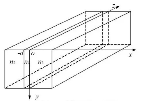
Three-layer planar slab waveguide To analyse planar slab optical waveguide using electromagnetic theory, the three-layer planar slab waveguide is simplified as that the electromagnetic field does not change in y-direction (
∂ ∂ y = 0 \frac{\partial}{\partial y}=0 ∂ y ∂ = 0 ). Thus, we can easily get one-dimensional wave equation of
E y E_y E y ,
∂ 2 E y ∂ x 2 + ( n j 2 k 2 − β 2 ) E y = 0 , j = 1 , 2 , 3 \frac{\partial^2E_y}{\partial x^2}+(n_j^2k^2-\beta^2)E_y=0,\quad j=1,2,3 ∂ x 2 ∂ 2 E y + ( n j 2 k 2 − β 2 ) E y = 0 , j = 1 , 2 , 3
Where k = 2 π / λ k=2\pi /\lambda k = 2 π / λ n j n_j n j n 1 > n 2 ≥ n 3 n_1>n_2\geq n_3 n 1 > n 2 ≥ n 3
E y = { A e − δ x , x ≥ 0 A cos ( κ x ) + B sin ( κ x ) , − d ≤ x ≤ 0 e γ ( x + d ) [ A cos ( κ d ) + B sin ( κ d ) ] , x ≤ − d E_y= \left\{ \begin{array}{lr} A\mathrm{e}^{-\delta x}, &x\geq0 \\ A\cos(\kappa x)+B\sin(\kappa x), &-d\leq x\leq 0 \\ \mathrm{e}^{\gamma(x+d)}[A\cos(\kappa d)+B\sin(\kappa d)], & x\leq -d \end{array} \right. E y = ⎩ ⎨ ⎧ A e − δ x , A cos ( κ x ) + B sin ( κ x ) , e γ ( x + d ) [ A cos ( κ d ) + B sin ( κ d )] , x ≥ 0 − d ≤ x ≤ 0 x ≤ − d
Where,
{ κ = n 1 2 k 2 − β 2 γ = β 2 − n 2 2 k 2 δ = β 2 − n 3 2 k 2 \left\{ \begin{array}{l} \kappa = \sqrt{n_1^2k^2-\beta^2} \\ \gamma = \sqrt{\beta^2-n_2^2k^2} \\ \delta = \sqrt{\beta^2-n_3^2k^2} \end{array} \right. ⎩ ⎨ ⎧ κ = n 1 2 k 2 − β 2 γ = β 2 − n 2 2 k 2 δ = β 2 − n 3 2 k 2
Since H z = i ω μ 0 ∂ E y ∂ x H_z=\frac{\mathrm{i}}{\omega \mu_0}\frac{\partial E_y}{\partial x} H z = ω μ 0 i ∂ x ∂ E y
H z = { − ( i δ / ω μ 0 ) A e − δ x , x ≥ 0 − ( i κ / ω μ 0 ) [ A sin ( κ x ) − B cos ( κ x ) ] , − d ≤ x ≤ 0 − ( i γ / ω μ 0 ) e γ ( x + d ) [ A cos ( κ d ) + B sin ( κ d ) ] , x ≤ − d H_z= \left\{ \begin{array}{lr} -(\mathrm{i}\delta /\omega\mu_0)A\mathrm{e}^{-\delta x}, &x\geq0 \\ -(\mathrm{i}\kappa /\omega\mu_0)[A\sin(\kappa x)-B\cos(\kappa x)], &-d\leq x\leq 0 \\ -(\mathrm{i}\gamma /\omega\mu_0)\mathrm{e}^{\gamma(x+d)}[A\cos(\kappa d)+B\sin(\kappa d)], & x\leq -d \end{array} \right. H z = ⎩ ⎨ ⎧ − ( i δ / ω μ 0 ) A e − δ x , − ( i κ / ω μ 0 ) [ A sin ( κ x ) − B cos ( κ x )] , − ( i γ / ω μ 0 ) e γ ( x + d ) [ A cos ( κ d ) + B sin ( κ d )] , x ≥ 0 − d ≤ x ≤ 0 x ≤ − d
According to the continuity conditions of electromagnetic waves at interfaces x = 0 x=0 x = 0 x = − d x=-d x = − d H z H_z H z
{ A δ + B κ = 0 A [ κ sin ( κ d ) − γ cos ( κ d ) ] + B [ κ cos ( κ d ) + γ sin ( κ d ) ] = 0 \left\{ \begin{array}{l} A\delta+B\kappa=0 \\ A[\kappa\sin(\kappa d)-\gamma\cos(\kappa d)]+B[\kappa\cos(\kappa d)+\gamma\sin(\kappa d)]=0 \\ \end{array} \right. { A δ + B κ = 0 A [ κ sin ( κ d ) − γ cos ( κ d )] + B [ κ cos ( κ d ) + γ sin ( κ d )] = 0
For the above system of linear equations of A A A B B B
δ [ κ cos ( κ d ) + γ sin ( κ d ) ] − κ [ κ sin ( κ d ) − γ cos ( κ d ) ] = 0 \delta[\kappa\cos(\kappa d)+\gamma\sin(\kappa d)]-\kappa[\kappa\sin(\kappa d)-\gamma\cos(\kappa d)]=0 δ [ κ cos ( κ d ) + γ sin ( κ d )] − κ [ κ sin ( κ d ) − γ cos ( κ d )] = 0
Multi Layer Slab Waveguide
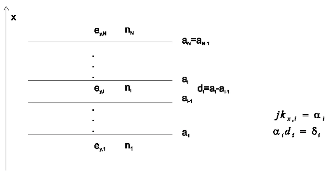
Multi layer slab waveguide Similarly, in layer i, continue working with the TE equation,
{ ∂ 2 E y , i ( x ) ∂ x 2 + k 0 2 n i 2 E y , i ( x ) = β 2 E y , i ( x ) ∂ ∂ x ( 1 k 0 2 n i 2 ∂ H y , i ( x ) ∂ x ) + H y , i ( x ) = β 2 k 0 2 n i 2 H y , i ( x ) \left\{ \begin{array}{l} \frac{\partial^2E_{y,i}(x)}{\partial x^2}+ k_0^2 n_i^2 E_{y,i}(x) = \beta^2 E_{y,i}(x)\\ \frac{\partial}{\partial x} \left( \frac{1}{ k_0^2n_i^2}\frac{ \partial H_{y,i}(x)}{\partial x} \right) + H_{y,i}(x) = \frac{\beta^2} {k_0^2 n_i^2} H_{y,i}(x) \end{array} \right. { ∂ x 2 ∂ 2 E y , i ( x ) + k 0 2 n i 2 E y , i ( x ) = β 2 E y , i ( x ) ∂ x ∂ ( k 0 2 n i 2 1 ∂ x ∂ H y , i ( x ) ) + H y , i ( x ) = k 0 2 n i 2 β 2 H y , i ( x )
The general solution to equation can be written as
E y , i = A i e i k x , i ( x − a i ) + B i e − i k x , i ( x − a i ) E_{y,i}=A_i \mathrm{e}^{\mathrm{i}k_{x,i}(x-a_i)}+B_i \mathrm{e}^{-\mathrm{i}k_{x,i}(x-a_i)} E y , i = A i e i k x , i ( x − a i ) + B i e − i k x , i ( x − a i )
Where k x , i = k 0 2 n i 2 − β 2 k_{x,i}=\sqrt{k_0^2n_i^2-\beta^2} k x , i = k 0 2 n i 2 − β 2
{ E y , i ( a i ) = E y , i + 1 ( a i ) ∂ E y , i ( a i ) ∂ x = ∂ E y , i + 1 ( a i ) ∂ x \left\{ \begin{array}{l} E_{y,i}(a_i)=E_{y,i+1}(a_i)\\ \frac{ \partial E_{y,i}(a_i)}{\partial x}=\frac{ \partial E_{y,i+1}(a_i)}{\partial x} \end{array} \right. { E y , i ( a i ) = E y , i + 1 ( a i ) ∂ x ∂ E y , i ( a i ) = ∂ x ∂ E y , i + 1 ( a i )
we can derive the following matrix relation:
[ A i B i ] = 1 2 α i ( ( α i + α i + 1 ) e − δ i + 1 ( α i − α i + 1 ) e δ i + 1 ( α i − α i + 1 ) e − δ i + 1 ( α i + α i + 1 ) e δ i + 1 ) [ A i + 1 B i + 1 ] \left[ \begin{array}{c} A_i \\ B_i \end{array} \right] = \frac{1}{2\alpha_i}\left( \begin{array}{cc} (\alpha_{i}+\alpha_{i+1})\mathrm{e}^{-\delta_{i+1}} & (\alpha_{i}-\alpha_{i+1})\mathrm{e}^{\delta_{i+1}} \\ (\alpha_{i}-\alpha_{i+1})\mathrm{e}^{-\delta_{i+1}} & (\alpha_{i}+\alpha_{i+1})\mathrm{e}^{\delta_{i+1}} \\ \end{array} \right) \left[ \begin{array}{c} A_{i+1} \\ B_{i+1} \end{array} \right] [ A i B i ] = 2 α i 1 ( ( α i + α i + 1 ) e − δ i + 1 ( α i − α i + 1 ) e − δ i + 1 ( α i − α i + 1 ) e δ i + 1 ( α i + α i + 1 ) e δ i + 1 ) [ A i + 1 B i + 1 ]
By repeating this procedure for all layers, the following matrix equation can be derived:
[ A 1 B 1 ] = ( t 11 ( β 2 ) t 12 ( β 2 ) t 21 ( β 2 ) t 22 ( β 2 ) ) [ A N B N ] \left[ \begin{array}{c} A_1 \\ B_1 \end{array} \right] = \left( \begin{array}{cc} t_{11}(\beta^2) & t_{12}(\beta^2) \\ t_{21}(\beta^2) & t_{22}(\beta^2) \end{array} \right) \left[ \begin{array}{c} A_{N} \\ B_{N} \end{array} \right] [ A 1 B 1 ] = ( t 11 ( β 2 ) t 21 ( β 2 ) t 12 ( β 2 ) t 22 ( β 2 ) ) [ A N B N ]
For guided modes
lim x → ± ∞ E y ( x ) = 0 \lim_{x \rightarrow \pm \infty}E_y(x)=0 x → ± ∞ lim E y ( x ) = 0
and because β > k 0 n N \beta > k_0n_N β > k 0 n N β > k 0 n 1 \beta > k_0n_1 β > k 0 n 1 A 1 = B N = 0 A_1 = B_N = 0 A 1 = B N = 0 t 11 ( β 2 ) = 0 t_{11}(\beta^2)=0 t 11 ( β 2 ) = 0
Reference 高等光学仿真(MATLAB版)- 光波导,激光(第3版) Optical-field calculations for lossy multiple-layer AlxGa1−xN/InxGa1−xN laser diodes Microphotonics (ugent.be)