The staggered finite-difference method

Why stagger the grid?

A staggered finite-difference method places selected unknowns at different spatial locations. This lets a difference between neighboring face values approximate a derivative at the cell center, while a difference between center values gives a derivative at a face. The layout is useful for first-order wave systems, where different field components are coupled through spatial derivatives.

I originally started this note with a one-dimensional acoustic model.^[1] The finite-cavity solver in our 3D-CWT repository now provides a concrete application: four optical envelopes live on cell faces, their coupling is evaluated at cell centers, and incoming boundary waves are eliminated exactly. This post connects the elementary stencil to that implementation. For the optical derivation, see CWT in PCSEL.

Spatial staggering in one dimension and the face-centered four-wave CWT layout

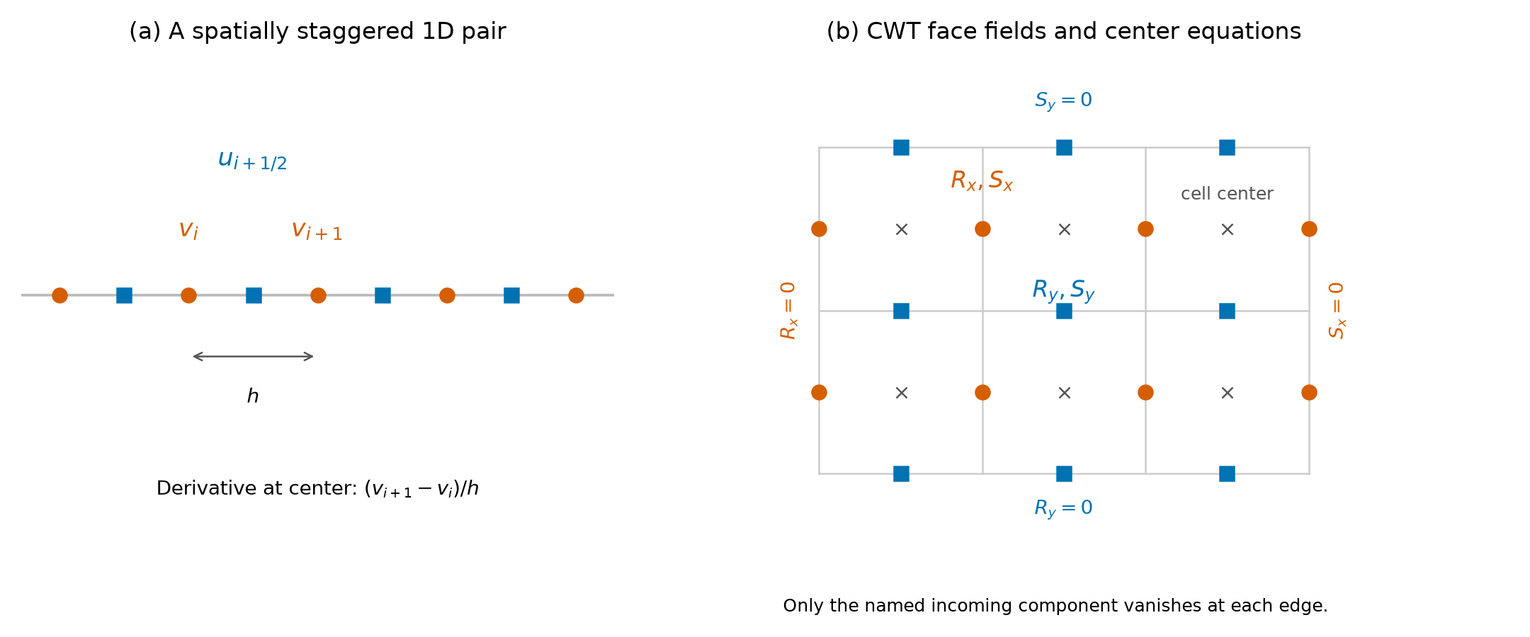
(a) A one-dimensional staggered pair. (b) The finite-CWT layout: orange circles carry $R_x,S_x$, blue squares carry $R_y,S_y$, and gray crosses mark the equation centers. Each boundary label constrains only the named incoming wave; the outgoing wave at the same location remains free.

One-dimensional problem

A first-order wave system

Consider the constant-speed system

$$\frac{\partial u}{\partial t}=c\frac{\partial v}{\partial x}, \qquad \frac{\partial v}{\partial t}=c\frac{\partial u}{\partial x}.$$

Here $u$ and $v$ are scaled wave variables and $c>0$ is the propagation speed. Eliminating either variable gives the wave equation, for example $u_{tt}=c^2u_{xx}$. The original normalized example corresponds to $c=1$.

Let the cell faces be $x_i=ih$, and the centers be $x_{i+1/2}=(i+1/2)h$. Store $v_i$ on faces and $u_{i+1/2}$ at centers. Then

$$\left.\frac{\partial v}{\partial x}\right|_{i+1/2} \approx\frac{v_{i+1}-v_i}{h}, \qquad \left.\frac{\partial u}{\partial x}\right|_i \approx\frac{u_{i+1/2}-u_{i-1/2}}{h}.$$

Although each expression uses two values, it is centered about the location where the derivative is evaluated. Taylor expansion about that midpoint gives

$$\frac{f(x+h/2)-f(x-h/2)}{h} =f'(x)+\frac{h^2}{24}f'''(x)+O(h^4).$$

The approximation is therefore second order for a smooth field. Its denominator is $h$, the distance between the two samples, not $2h$.

One motivation is the grid-scale alternating pattern $v_i=(-1)^i$. A collocated centered derivative $(v_{i+1}-v_{i-1})/(2h)$ vanishes on this pattern, while the staggered derivative $(v_{i+1}-v_i)/h$ does not. Staggering changes the derivative’s discrete nullspace; boundary treatment and the complete coupled operator still require their own checks.

Optional staggering in time: leapfrog

For explicit wave propagation, also place $u$ at integer times and $v$ at half times:

$$\begin{aligned} u_{i+1/2}^{n+1} &=u_{i+1/2}^{n} +\frac{c\Delta t}{h}\left(v_{i+1}^{n+1/2}-v_i^{n+1/2}\right),\\ v_i^{n+3/2} &=v_i^{n+1/2} +\frac{c\Delta t}{h}\left(u_{i+1/2}^{n+1}-u_{i-1/2}^{n+1}\right). \end{aligned}$$

The two updates alternate, each using values at the other variable’s latest time level. Half-time initial data must be supplied consistently, for example through a half-step from the prescribed initial fields.

For a uniform infinite or periodic grid, Fourier analysis gives

$$\sin^2\left(\frac{\omega\Delta t}{2}\right) =\left(\frac{c\Delta t}{h}\right)^2 \sin^2\left(\frac{kh}{2}\right).$$

For unrestricted staggered initial data, a sufficient stability condition is $c\Delta t/h<1$. The familiar upper bound $c\Delta t/h\le1$ follows from the real-frequency condition, but equality needs separate treatment: when the grid admits the Nyquist mode, its amplification matrix has a nontrivial Jordan block and generic initial data can grow linearly in the step count. Space and time staggering are separate choices: the CWT eigenproblem below uses the spatial layout without this leapfrog time update.

Two-dimensional problem

A two-dimensional wave system needs two directional components:

$$\begin{aligned} u_t&=c\left(\partial_xv_x+\partial_yv_y\right),\\ (v_x)_t&=c\,\partial_xu,\\ (v_y)_t&=c\,\partial_yu. \end{aligned}$$

Use $u_{i+1/2,j+1/2}$ at cell centers, $(v_x)_{i,j+1/2}$ at $x$ faces, and $(v_y)_{i+1/2,j}$ at $y$ faces. The discrete divergence is

$$(\nabla_h\cdot\mathbf v)_{i+1/2,j+1/2} =\frac{(v_x)_{i+1,j+1/2}-(v_x)_{i,j+1/2}}{h_x} +\frac{(v_y)_{i+1/2,j+1}-(v_y)_{i+1/2,j}}{h_y}.$$

The corresponding gradient at an $x$ face is

$$(\partial_x^hu)_{i,j+1/2} =\frac{u_{i+1/2,j+1/2}-u_{i-1/2,j+1/2}}{h_x},$$

with the analogous expression at a $y$ face. These differences connect face and center grids naturally. For the constant-speed explicit leapfrog scheme on a uniform periodic grid, a sufficient two-dimensional CFL condition is

$$c^2\Delta t^2\left(\frac{1}{h_x^2}+\frac{1}{h_y^2}\right)<1.$$

The equality endpoint has the same critical-mode qualification as in one dimension. Boundary conditions must match the underlying wave problem. A closed acoustic boundary and an open optical aperture impose different conditions even when their variable locations look similar.

Application: the finite-cavity CWT equations

Four envelopes and four transport directions

For the square-lattice TE model, write the slowly varying envelopes as

$$\mathbf V=(R_x,S_x,R_y,S_y)^{\mathsf T}.$$

The finite-domain equations are^[2]

$$\Lambda\mathbf V=C\mathbf V+\mathrm{i} \begin{pmatrix} \partial_xR_x\\-\partial_xS_x\\ \partial_yR_y\\-\partial_yS_y \end{pmatrix}, \qquad \Lambda=\delta+\mathrm{i}\alpha.$$

$C$ is a uniform $4\times4$ coupling matrix calculated from the vertical waveguide and photonic-crystal geometry. Here $\beta_0=2\pi/a$, with lattice period $a$, and $\delta=(\beta^2-\beta_0^2)/(2\beta_0)\simeq\beta-\beta_0$ is the linearized Bragg detuning of the reference guided propagation constant $\beta$. In the package, lengths are in µm, while $C$, $\delta$, and $\alpha$ have units µm⁻¹. The convention is $\exp(+\mathrm{i}\omega t)$, and $\alpha$ is an amplitude-loss coefficient; power loss uses $2\alpha$. Thus $\Lambda$ is not a complex angular frequency, and $\alpha$ is not a temporal decay rate.

Unlike the acoustic example, this is a stationary eigenvalue problem. We reuse the face–center discretization structure, not derive the optical equations from the acoustic system. Spatially staggering the envelopes does not introduce a time step or a CFL condition into its solution.

Locations, array shapes, and incoming boundaries

Divide $[0,L_x]\times[0,L_y]$ into $N_x\times N_y$ cells:

$$h_x=L_x/N_x,\qquad h_y=L_y/N_y.$$

Store the fields as follows. NumPy arrays use row $=y$, column $=x$.

Field	Location	Full array shape	Fixed incoming boundary
$R_x$	$(x_i,y_{j+1/2})$	(Ny, Nx+1)	Rx[:, 0] = 0
$S_x$	$(x_i,y_{j+1/2})$	(Ny, Nx+1)	Sx[:, -1] = 0
$R_y$	$(x_{i+1/2},y_j)$	(Ny+1, Nx)	Ry[0, :] = 0
$S_y$	$(x_{i+1/2},y_j)$	(Ny+1, Nx)	Sy[-1, :] = 0

For example, the left boundary fixes $R_x$, but leaves $S_x$ free to leave the cavity. Applying zero to both would change the open-boundary problem.

The free arrays are Rx[:, 1:], Sx[:, :-1], Ry[1:, :], and Sy[:-1, :]. Each has $N_xN_y$ entries, giving exactly

$$n_{\mathrm{dof}}=4N_xN_y$$

free complex amplitudes and the same number of cell-centered equations. The implementation packs them component by component in the order $(R_x,S_x,R_y,S_y)$, flattening each block in C order. Incoming values are omitted from the unknown vector and restored as exact zeros when reconstructing fields; there are no penalty constants or extra corner variables.

These cells resolve the slow cavity envelope, not the individual photonic-crystal periods. $N_x$ and $N_y$ are numerical controls, not counts of unit cells in the physical device.

Average the field; difference the transport

Every local coupling term needs all four fields at the same cell center. In the expressions below, center subscripts $i,j$ label the cell at $(x_{i+1/2},y_{j+1/2})$. For example,

$$\bar R_{x;i,j} =\frac{R_{x;i,j+1/2}+R_{x;i+1,j+1/2}}{2},$$

$$(D_xR_x)_{i,j} =\frac{R_{x;i+1,j+1/2}-R_{x;i,j+1/2}}{h_x}.$$

Use the same average for $S_x$, but reverse the derivative sign. For $R_y,S_y$, average bottom and top faces and difference along $y$, again reversing the sign for $S_y$.

For any component $f$, the adjacent-face average satisfies

$$\frac{f(x-h/2)+f(x+h/2)}{2} =f(x)+\frac{h^2}{8}f''(x)+O(h^4).$$

Both the interpolation and the derivative are second order. The local $R_x$ equation is therefore

$$\Lambda\bar R_{x;i,j} =\sum_{\ell=1}^4 C_{1\ell}\bar V_{\ell;i,j} +\mathrm{i}\frac{R_{x;i+1,j+1/2}-R_{x;i,j+1/2}}{h_x}.$$

The eigenvalue multiplies the average, not one of the face values. This distinction produces the matrix $B$ in the generalized problem.

Sparse assembly: $Av=\Lambda Bv$

Let $v$ contain the free face amplitudes; this packed optical vector is unrelated to the earlier acoustic variable $v$. Define $Bv$ as the stacked cell-center averages and $Dv$ as the stacked signed differences. With component-major ordering, let $C_{\mathrm{lift}}=C\otimes I_{N_xN_y}$ denote application of the same local coupling to every cell. Then

$$A=C_{\mathrm{lift}}B+\mathrm{i}D, \qquad Av=\Lambda Bv.$$

This Kronecker product describes the operator mathematically; the implementation assembles local sparse triplets directly without constructing a dense lifted matrix.

For each retained face, averaging contributes $1/2$. A difference contributes $\pm1/h_x$ or $\pm1/h_y$, with the transport sign of its component. Coupling into receiver equation $r$ contributes $C_{r\ell}/2$. When a face is a prescribed incoming zero, its column is simply omitted.

For a four-cell $x$ row, the averaging blocks are

$$B_{R_x}=\frac12 \begin{pmatrix} 1&0&0&0\\ 1&1&0&0\\ 0&1&1&0\\ 0&0&1&1 \end{pmatrix}, \qquad B_{S_x}=B_{R_x}^{\mathsf T}.$$

Thus $B$ is an interpolation operator and is generally non-Hermitian, even though it is square. On this boundary-eliminated layout its blocks are triangular with nonzero diagonal, so $B$ is invertible. It is not the symmetric positive-definite mass matrix assumed by some generalized eigensolver interfaces.

For a generic fully populated $C$, the local stencil gives at most eight nonzeros per row of $A$, and at most two per row of $B$. Assembly and sparse storage scale linearly with $N_xN_y$. Sparse LU factorization can have additional fill-in; linear assembly storage does not imply linear eigensolve cost.

A one-cell check

A single cell has four free outgoing values and four incoming zeros. Its matrices are

$$B=\frac12I_4, \qquad D=\operatorname{diag}\left(h_x^{-1},h_x^{-1},h_y^{-1},h_y^{-1}\right),$$

$$A=\frac12C+\mathrm{i}D.$$

All four diagonal entries of $D$ are positive here. For $S_x$, for instance, the signed difference is $-(0-S_{x,\mathrm{left}})/h_x$. This tiny example checks transport signs, averaging factors, and boundary elimination before any large solve.

Shift-invert without forming $B^{-1}$

To find eigenvalues near a complex target $\sigma$, require $A-\sigma B$ to be invertible and use

$$T=(A-\sigma B)^{-1}B.$$

An eigenpair $Tv=\mu v$ gives

$$\Lambda=\sigma+\frac{1}{\mu}.$$

The code factors the sparse matrix $A-\sigma B$ once, exposes $T$ as a linear operator, and calls ARPACK through SciPy. It does not form a dense inverse or blindly pass this non-Hermitian $B$ as an SPD mass matrix.

The returned vector is checked against the original pencil using

$$\eta=\frac{\|Av-\Lambda Bv\|_2} {\left(\|A\|_F+|\Lambda|\|B\|_F\right)\|v\|_2}.$$

A small residual shows that the approximate eigenpair satisfies the original discrete equations to the stated tolerance. It does not by itself bound eigenvalue forward error for a non-normal or nearly defective pencil. Mesh refinement is a separate test of how that discrete problem approximates the continuous one. A targeted search also covers only the modes near its selected shift.

A discrete power identity

The face-average construction has an exact telescoping property. For complex face values $a,b$,

$$2\operatorname{Re}\left[ \left(\frac{a+b}{2}\right)^*\frac{b-a}{h}\right] =\frac{|b|^2-|a|^2}{h}.$$

Summing over cells cancels every interior face contribution. Write $U=Bv$ and define

$$\begin{aligned} P_{\mathrm{edge}}={}&h_y\sum_j\left( |R_x(L_x,y_{j+1/2})|^2+|S_x(0,y_{j+1/2})|^2\right)\\ &+h_x\sum_i\left( |R_y(x_{i+1/2},L_y)|^2+|S_y(x_{i+1/2},0)|^2\right). \end{aligned}$$

The exact discrete identity is

$$2h_xh_y\operatorname{Im}\left[ U^\dagger\left(Av-C_{\mathrm{lift}}U\right)\right] =P_{\mathrm{edge}}.$$

It holds for any free complex vector, not only an eigenmode, so it can test assembly independently of the eigensolver. For an eigenmode, define $P=h_xh_y\|U\|_2^2$ to obtain

$$2\alpha P=P_{\mathrm{edge}} +2h_xh_y\operatorname{Im}\left(U^\dagger C_{\mathrm{lift}}U\right).$$

A Hermitian $C$ makes the volume term vanish. For the optical coupling matrix, its anti-Hermitian part accounts for open radiation channels under the model’s stated conditions. For an arbitrary complex test matrix, keep this as a signed coupling contribution rather than automatically calling it radiated power.

The package normalizes reconstructed modes to $P=1$. These quantities are envelope norms and loss budgets; they are not calibrated optical powers in watts. The plotted envelope intensity is the cell-centered sum $|R_x|^2+|S_x|^2+|R_y|^2+|S_y|^2$, without the fast unit-cell interference pattern.

Verification with smooth manufactured fields

To test spatial accuracy independently of an eigensolver, prescribe smooth complex fields satisfying the incoming zeros. On a $30\times20\ \mu\mathrm m^2$ rectangle, use

$$\begin{aligned} R_x&=a_1(x/L_x)^3(1+0.2y/L_y),\\ S_x&=a_2(1-x/L_x)^3(1+0.2y/L_y),\\ R_y&=a_3(y/L_y)^3(1+0.2x/L_x),\\ S_y&=a_4(1-y/L_y)^3(1+0.2x/L_x), \end{aligned}$$

with $(a_1,a_2,a_3,a_4)=(1+2\mathrm{i},2-\mathrm{i},-0.5+\mathrm{i},3+0.7\mathrm{i})$. Sample these fields on faces and compare the assembled averages and derivatives with their analytic values at cell centers.

For the full operator, use the deliberately illustrative Hermitian matrix

$$C=\begin{pmatrix} 0&0.02&0.01&0.01\\ 0.02&0&0.01&0.01\\ 0.01&0.01&0&0.02\\ 0.01&0.01&0.02&0 \end{pmatrix}\ \mu\mathrm m^{-1}.$$

This matrix is a numerical test input, not a coupling matrix extracted from a particular PCSEL. Define each relative error as the Euclidean norm of the discrete-minus-analytic vector divided by the norm of its analytic reference. The full-operator comparison uses $Av$ against the analytic center samples of

$$C\mathbf V+\mathrm{i}(\partial_xR_x,-\partial_xS_x,\partial_yR_y,-\partial_yS_y)^{\mathsf T}.$$

No eigenvalue is solved for these prescribed fields. For $N_x=N_y=N$, actual execution of package version 1.4.0 gives:

$N$	Center-average error	Signed-derivative error	Full-operator error
8	1.81128 × 10⁻²	2.93064 × 10⁻³	4.44798 × 10⁻³
16	4.48832 × 10⁻³	7.29074 × 10⁻⁴	1.10709 × 10⁻³
32	1.11961 × 10⁻³	1.82046 × 10⁻⁴	2.76467 × 10⁻⁴
64	2.79749 × 10⁻⁴	4.54975 × 10⁻⁵	6.90978 × 10⁻⁵

Measured second-order refinement of the actual staggered CWT spatial operators

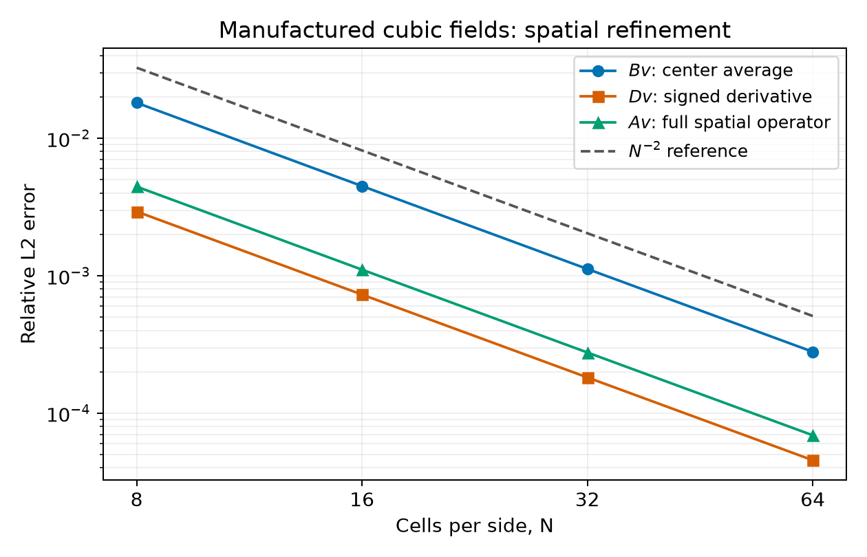
Relative errors of center averaging, signed differentiation, and the full spatial operator. The dashed line is an $N^{-2}$ reference. These are manufactured-field consistency checks, not physical-device eigenmode results.

The observed orders $\log_2(e_N/e_{2N})$ range from 2.0004 to 2.0128 over these refinements. Separately, random complex vectors on the same grids satisfy the outgoing-flux identity to relative errors below $3\times10^{-16}$ in this run. The first test measures spatial truncation; the second checks the discrete algebra. Neither replaces Fourier-cutoff convergence of the optical coupling or tracking the same physical eigenmode across cavity grids.

A runnable Python example

Install the matching package with python -m pip install cwt3d==1.4.0. The following example uses the same illustrative matrix to exercise the actual sparse assembler, eigensolver, and field reconstruction:

import numpy as np
from cwt3d.finite import (
    StaggeredGrid, assemble_pencil, solve_finite, reconstruct_modes,
)

# Synthetic test coupling in um^-1, not a device-derived optical matrix.
C = np.array([
    [0, 0.02, 0.01, 0.01],
    [0.02, 0, 0.01, 0.01],
    [0.01, 0.01, 0, 0.02],
    [0.01, 0.01, 0.02, 0],
], dtype=complex)

grid = StaggeredGrid(Nx=16, Ny=12, Lx_um=30, Ly_um=20)
pencil = assemble_pencil(grid, C)
result = solve_finite(
    pencil, sigma=-0.03 + 0.04j, k=3,
    tol=1e-10, residual_tol=1e-9, seed=33,
)
modes = reconstruct_modes(pencil, result)

assert grid.n_dof == 4 * 16 * 12
for mode in modes:
    assert mode.boundary_error == 0
    assert mode.residual < 1e-9
    assert mode.budget["balance_relative_error"] < 1e-10
    print(mode.delta, mode.alpha, mode.residual)
    print("edge loss:", mode.budget["edge"])
    print("center field:", mode.centers.Rx.shape)

The run returns three modes, each with center arrays of shape (12, 16). Because $C$ is Hermitian, the nonzero $\alpha$ comes from the outgoing boundaries and the edge budget equals $2\alpha$ after normalization. To calculate a device, replace this test matrix with coupling.C from the optical pipeline described in the repository’s API guide.

The implementation is separated into grid and boundary indexing, sparse assembly, targeted eigensolving, and field reconstruction and power budgets. The assembly tests include independent small-matrix, manufactured-field, and outgoing-flux checks.

References

---

1. The staggered finite-difference method (交错网格有限差分方法), 数值分析大巴. The one- and two-dimensional wave examples motivate the introductory sections; the indexing convention here places $u$ at cell centers. ↩︎

2. Y. Liang, Three-dimensional coupled-wave theory for photonic-crystal surface-emitting lasers, doctoral thesis, Kyoto University. DOI: 10.14989/doctor.k18283. Chapter 4, Eqs. (4.21)–(4.22), gives the finite-envelope equations and no-incoming-wave boundary conditions. ↩︎